Automatic sound programming: first results
·This post presents early results for the Secret Sauce project. We show that it is possible to predict guitar effects accurately with high level audio features and recurrent neural nets, but predicting synthesizer patches is more challenging.
Note: this is the second post on automatic sound programming. For an overview of the project, check out the first one.
Introduction
The aim of the Secret Sauce project is to automatically reverse engineer sounds: give the model a sample, and it tells you how to approximate it with a synthesizer or a set of guitar effects. But how hard is the task?
This post presents our first results, based on the Guitar Effect and Noisemaker datasets. Some results are positive, others are negative—the aim here is to give an idea of what we can achieve with a few days work and set a baseline for future research.
All the models are based on Scikit learn and Keras with Tensorflow as back-end. We used heavily rely on the librosa library for feature extraction. Our code is available on Github.
The Models
The Secret Sauce task is interesting for two reasons. First, its input is a collection of 10,000 waveforms, each containing more than 19,000 points. Given the high dimensionality of the dataset and the (relatively) small size of the collection, feeding the raw data to the algorithms is likely to be inaccurate and inefficient — we need more compact features.
Second, Secret Sauce is a joint modeling task, where we wish to predict several variables at the same time. Because the variables have different types, we model the problem as a mix of regression (for the knobs) and classification (for the switches). In some cases, the objective interact with each other: in the guitar case for instance, the parameters associated to effects that are disabled have no impact on the final sound an should be ignored. We will see that neural networks provide a clean way to model those dependencies.
Sound representation
Inspired by the music analysis literature, we model sound with two types of representations: Mel-scaled spectrograms and Mel Frequency Cepstral Coefficients (MFCCs) [1]. The former is a spectrogram rescaled to match human perception. We call it a mid-level feature because it is close to the raw sound [2]. The latter is a high level feature, obtained by computing the spectrum of the spectrum — you may think of the MFCCs as a compact, decorrelated version of the Mel spectrogram, shown to very successful for speech recognition [3,4]. We used librosa’s implementation for both methods.
To get a better intuition for what those features represent, let us plot them. This is the waveform of sample #22 in the Noisemaker light dataset:
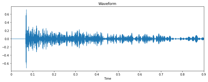
The waveform is the lowest level of representation available. In this example, it shows that the sound has a strong attack and a weak sustain, and the fact that the curve is unpredictably “wiggly” indicates the presence of white noise. Those characteristics are typical of percussive sounds.
The Mel spectrogram gives more insight into the sound’s timbre:
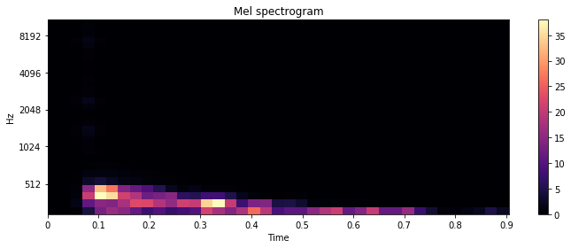
In this case, we perceive a streak at the bottom and emptiness everywhere else. This reveals that the sound is heavily filtered.
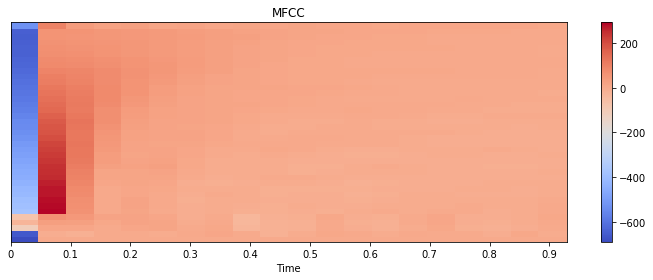
The MFCCs are harder to interpret. We perceive the dynamics of the sample (first a blank, then an attack, then the thin sustain), but it is difficult to learn more about its timbre.
After seeing all those plots, you may wonder what the original sample sounds like. Here it is:
We provide the details of feature extraction in Appendix 1.
Models
We compare two types of models. In independent models, we treat each target as a separate inference problem, thus we train one predictor for each variable. We tried three types of algorithms: k-Nearest Neighbors, decision/regression trees and a naive baseline which predicts the majority class (for classification) or the average (for regression). We tuned the algorithms with cross-validation, with one distinct set of parameters for every variable.
Joint models predict all the variables with one algorithm, in this case a neural network. The hope is that sharing the representation of the input across the tasks will improve the accuracy of the predictions, as often shown in the deep learning literature [5]. We use 1D convolutional NNs, LSTMs and fully connected NNs with several layers and multiplicative connections to model the dependency between the outputs. We use a held-out validation set to chose the parameters, see details in appendices 2 and 3.
Results
Metrics
In what follows, we report two metrics: the mean absolute error (MAE) for regression and the accuracy for classifications, both averaged across the variables of the same type. We use the first 80% of the data for training and validation, and the remaining 20% for testing. In the guitar case, we only report the scores for the effects that are enabled.
Guitar Dataset
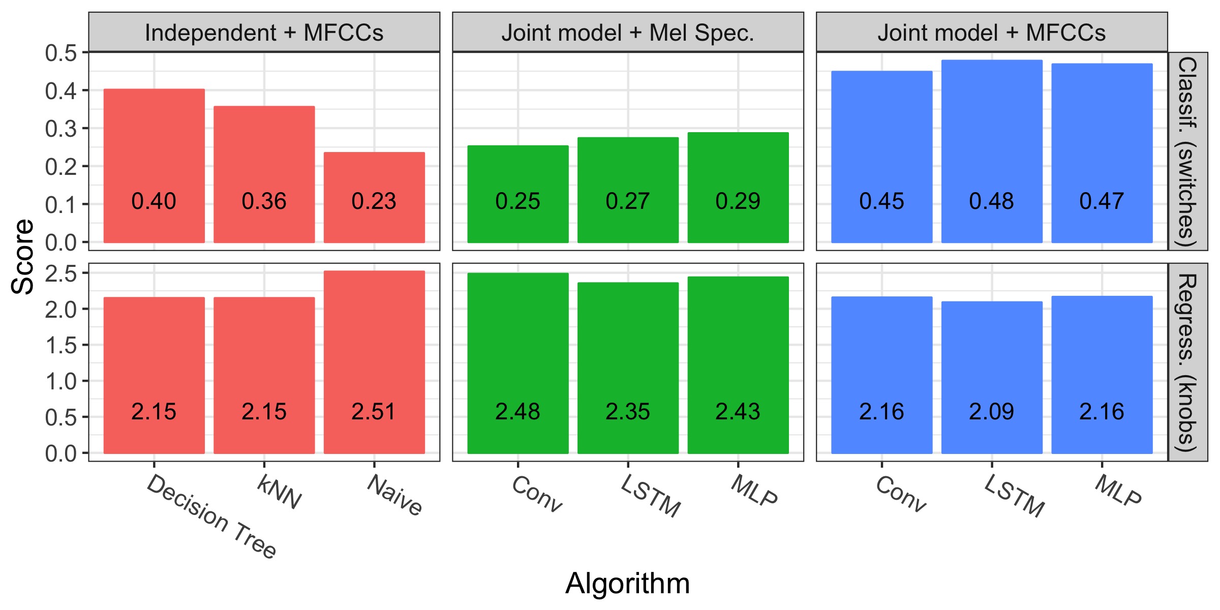
The figure below presents our results for the Guitar Effect dataset. The top line presents the classification scores (higher is better), the low line presents the regression scores (lower is better).
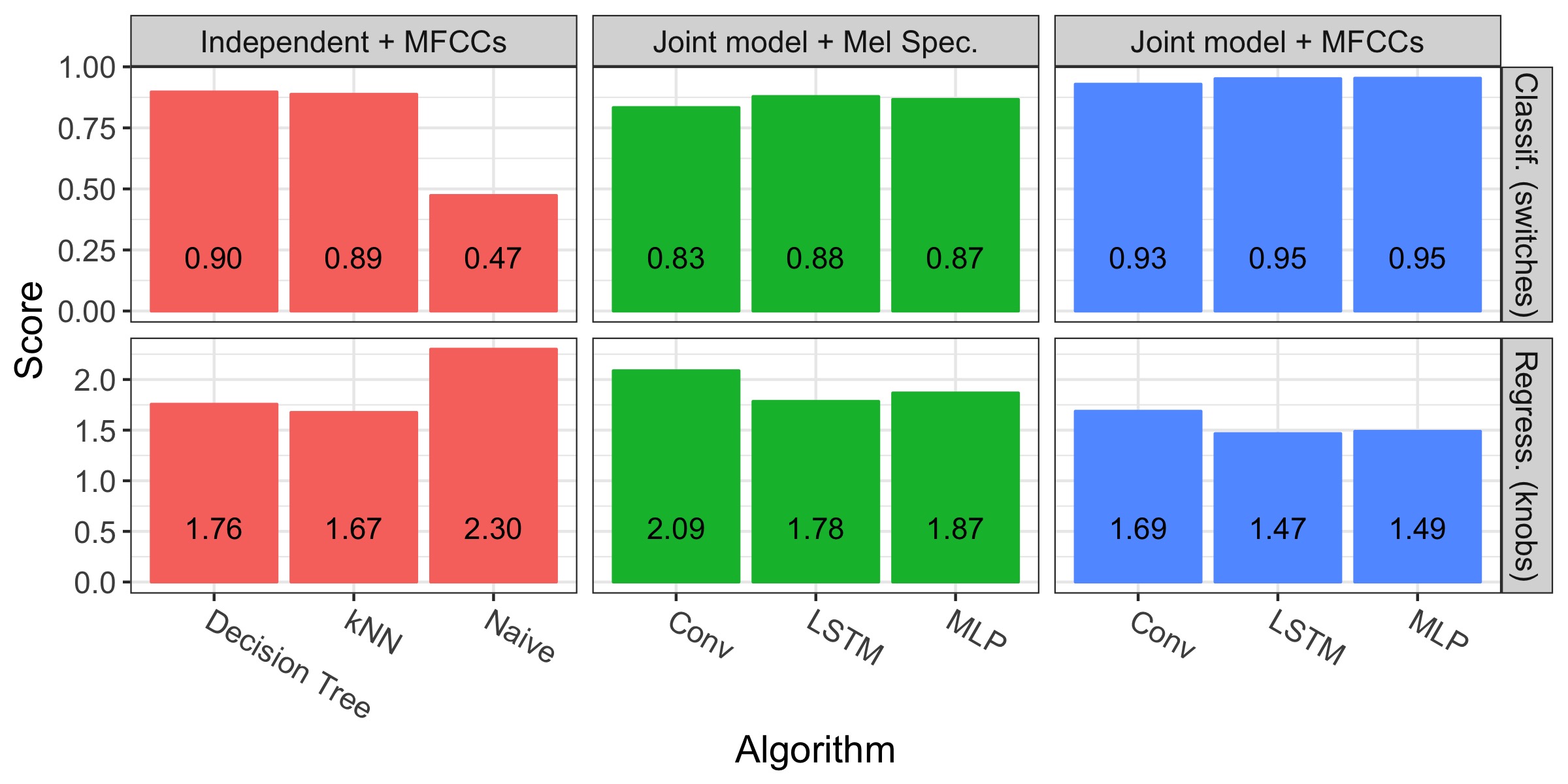
Let us examine the Naive strategy. The classification accuracy is close to 0.5 because all the categorical variables are binary and uniformly sampled. Similarly, the MAE is close to 2.5 because the knob values are sampled between 0 and 10 and the naive regressor always predicts the mean (5). Those numbers pass the sanity check.
On the overall, the classification scores are excellent, indicating that our models can predict which effects are enabled with high accuracy. Predicting the continuous variables seems more difficult, as the algorithms are up to 2.09 ticks off the true values (out of 10). Fortunately, those inaccuracies have only little impact on the final sound. To get a better intuition for their magnitude, let us listen to a few samples. In the following video, we play the first 15 notes from the test set, followed by the predictions of the LSTM (the best model we have). Can you hear the difference?
The LSTM + MFCCs approach outperforms all the others, closely followed by MLP. The independent approaches provide good results too. In contrast, the mid-level features lead to poor results; we hypothesize that this is due to the small size of the dataset. The neural networks do not have the resources to learn good representations, therefore they work better with high level features.
Noisemaker Dataset
We now present the scores for the Noisemaker dataset:
We see that the models perform better than the baseline, but the metrics are rather weak on the overall. How much does this matter? After all, inaccuracies are acceptable if they are imperceptible to humans. To verify, we compare the first 15 samples of the test set to the LSTM’s predictions:
We hear that in most cases, the predictor captures the “spirit” of the sound, but it does not get the details right. Therefore, our conclusion are mixed: the models do help reverse-engineering the sounds, but the results are not perfect.
As previously, it seems that classification is slightly less difficult than regression, and that joint models over MFCCs dominate the other approaches. To understand what the predictor got wrong, we investigated each target variable individually. We found that almost all models struggle with the parameters related to dynamics and long term properties of the sound (e.g., envelopes and LFOs), which calls for better features. Appendix 4 presents more details.
Other Datasets
You may find Jupyter notebooks for all the other datasets in our Github repository. In short, we obtain satisfying results with similar methods on the small datasets (Noisemaker light and Guitar Effects light), but the results for the Moog collection are worse than those for Noisemaker.
Conclusion and Plan of Action
This blog post described our first set of experiments with the Guitar and Noisemaker datasets. The conclusions are mixed: we modeled the guitar effect dataset successfully, but found that the Noisemaker task harder to solve.
The next step is to try better features. First, we will try to combine the MFCCs with other features from the literature, such as deltas and constant-Q representations. Then, we will scale our experiment up and generate more data so that the algorithms can learn features themselves. To be continued!
References
[1] “An exploration of deep learning in content-based music informatics”, PhD thesis, EJ Humphrey - 2015 link
[2] “End-to-End Learning for Music Audio”, Dieleman and Schrauwen, IEEE International Conference on Acoustic Speech and Signal Processing (ICASSP); 2016 link
[3] “Design, analysis and experimental evaluation of block based transformation in MFCC computation for speaker recognition”, Sahidullah and Saha; Speech Communication; 2012
[4] “Mel Frequency Cepstral Coefficients for Music Modeling”, Beth Logan; International Symposium on Music Information Retrieval; 2000
[5] “Multi-task learning in deep neural networks for improved phoneme recognition”, Seltzer and Droppo; IEEE ICASSP; 2013
Appendix 1: Detail of the Feature Extraction
For all the datasets, we convert the samples to 22,050Hz and use windows of width 2048 with jumps of 512 frames. We use 20 MFCCs and 32 Mel bins.
Apendix 2: Detail of the Neural Networks
All the models have the same outputs: softmax layers with cross-entropy for the switches and fully connected layer with MSE loss for the knobs. We model the dependencies between the on/off switches of the effects and their parameters with multiplicative connections — for instance, in the guitar effect case, we multiply the predicted distortion rate with the binary variable that indicates whether the distortion is enabled or not.
For the convolutional layer, we used a window of size 4 and stride 1. Each convolution layer is followed by 1D max pooling with window size 4 and stride 2. We set the number of filters at layer i to be #filters * i to create a VGG-like pyramidal structure.
We used the optimizer Adam, with the default parameters of Keras. We use 50 epochs, but stop the training when the validation does not improve after 5 epochs.
We tried L2 regularization over the weights of all the models without success.
Even more details in the source code.
Appendix 3: Topology of the Neural Networks
| Representation | Algorithm | Parameter | Guitar | Noisemaker |
|---|---|---|---|---|
| Mel spec. | MLP | #hidden units | 128 | 64 |
| Mel spec. | MLP | #layers | 2 | 2 |
| MFCC | MLP | #hidden units | 128 | 128 |
| MFCC | MLP | #layers | 1 | 2 |
| Mel spec. | LSTM | #hidden units | 80 | 80 |
| Mel spec. | LSTM | #layers | 2 | 2 |
| MFCC | LSTM | #hidden units | 128 | 128 |
| MFCC | LSTM | #layers | 2 | 2 |
| Mel spec. | Conv | #filters | 64 | 16 |
| Mel spec. | Conv | #layers | 2 | 1 |
| MFCC | Conv | #filters | 48 | 64 |
| MFCC | Conv | #layers | 2 | 2 |
Appendix 4: Detail of the MFCC+LSTM scores on the Noisemaker dataset
Not all predictions are bad for the Noisemaker dataset. Let us inspect the results for each task separately.
Classification
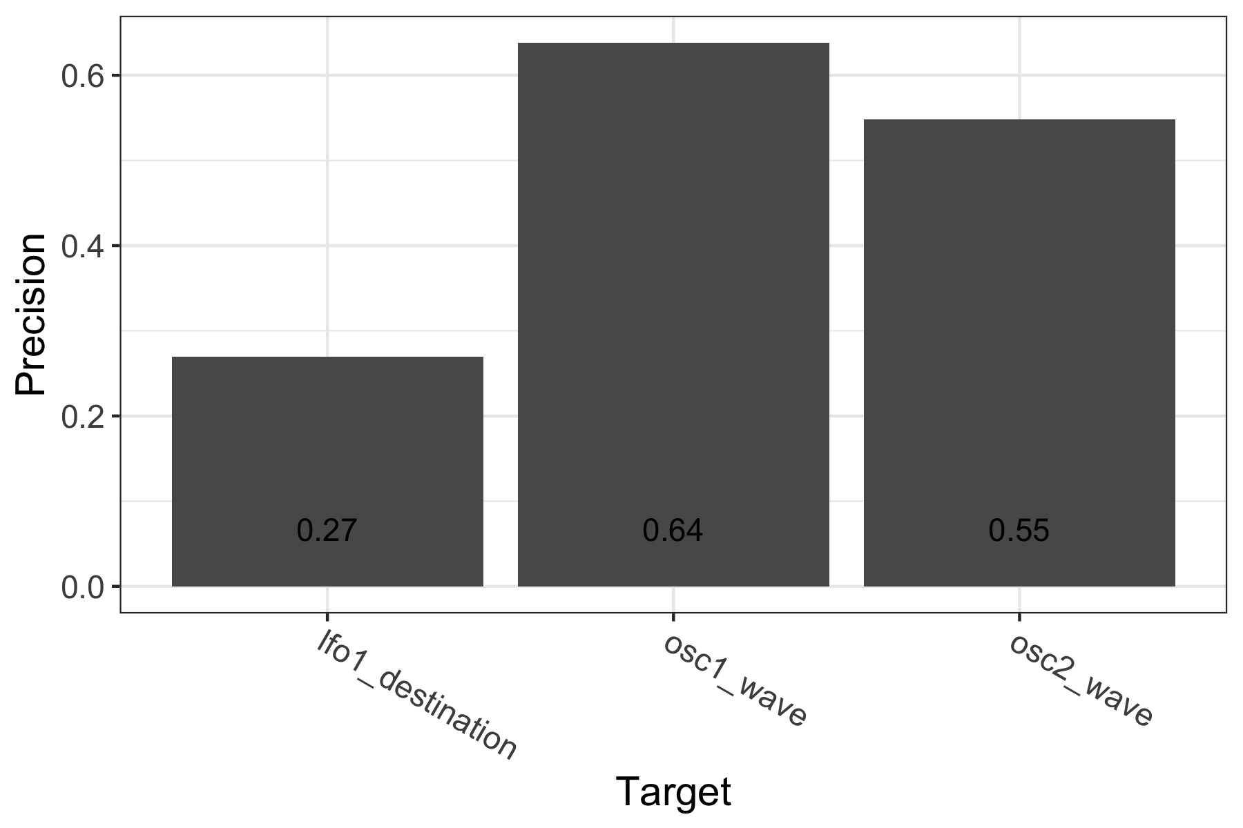
The LSTM can predict the oscillator waveforms with mediocre, but not catastrophic accuracy. However, the LFO destination is much harder to model.
Regression
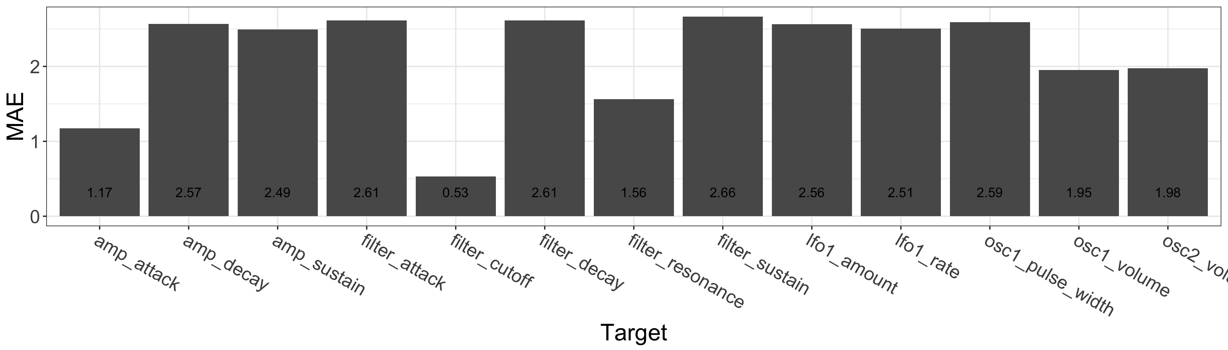
The LSTM gets a few parameters right: the filter cutoff and resonance, the amp attack, and to a lesser extent the mix between the oscillators. Problems appear with the other envelope parameters and the LFO settings. Those targets relate to dynamics, which calls for investigations into more appropriate features.